The Iris dataset is a classic in the field of machine learning and statistics. It’s often used for practicing classification algorithms. The dataset contains 150 samples of iris flowers, each with four features: sepal length, sepal width, petal length, and petal width. The samples are evenly distributed across three species of iris flowers: Setosa, Versicolor, and Virginica. In this article we shall perform data analysis of Iris dataset using Python.
Steps for Data Analysis of Iris Dataset
- Step 1: Data Loading
- Step 2: Data Exploration
- Step 3: Data Visualization
- Step 4: Statistical Summary
- Step 5: Correlation Analysis of Iris Dataset
Here are the steps we’ll follow for the complete data analysis of Iris dataset:
- Data Loading: Load the Iris dataset.
- Data Exploration: Explore the dataset to understand it better and figure out how to approach the classification problem.
- Data Visualization: Visualize the data to understand the relationships between features and species.
- Statistical Summary: Summarize the data statistically to extract insights.
- Correlation Analysis: Understand how features correlate with each other.
Let’s get started!
Package required: sklearn
Step 1: Data Loading
First, let’s load the Iris dataset.
from sklearn.datasets import load_iris
import pandas as pd

# Load the Iris dataset
iris_data = load_iris()
iris_df = pd.DataFrame(iris_data.data, columns=iris_data.feature_names)
iris_df['species'] = iris_data.target_names[iris_data.target]

# Show first few rows of the dataset
iris_df.head()
Output:
sepal length (cm)	sepal width (cm)	petal length (cm)	petal width (cm)	species
5.1	                3.5	              1.4	                0.2	          setosa
4.9	                3.0	              1.4	                0.2	          setosa
4.7	                3.2	              1.3	                0.2	          setosa
4.6	                3.1	              1.5	                0.2	          setosa
5.0	                3.6	              1.4	                0.2	          setosa
The dataset has been successfully loaded. It contains four feature columns:
- Sepal length (cm)
- Sepal width (cm)
- Petal length (cm)
- Petal width (cm)
Additionally, it has a ‘species’ column, which is the label we would typically predict in a machine learning task.
Step 2: Data Exploration
Let’s start by checking for any missing values and understanding the basic statistics of the dataset.
# Check for missing values
missing_values = iris_df.isnull().sum()

# Basic statistics of the dataset
statistics_summary = iris_df.describe()

missing_values, statistics_summary
Oytput:
(sepal length (cm)    0
 sepal width (cm)     0
 petal length (cm)    0
 petal width (cm)     0
 species              0
 dtype: int64,
        sepal length (cm)  sepal width (cm)  petal length (cm)  \
 count         150.000000        150.000000         150.000000
 mean            5.843333          3.057333           3.758000
 std             0.828066          0.435866           1.765298
 min             4.300000          2.000000           1.000000
 25%             5.100000          2.800000           1.600000
 50%             5.800000          3.000000           4.350000
 75%             6.400000          3.300000           5.100000
 max             7.900000          4.400000           6.900000

        petal width (cm)
 count        150.000000
 mean           1.199333
 std            0.762238
 min            0.100000
 25%            0.300000
 50%            1.300000
 75%            1.800000
 max            2.500000  )
Great! There are no missing values in the dataset, which simplifies things for us.
Here are some basic statistics for each of the feature columns:
- Sepal length (cm): Ranges from 4.3 to 7.9 with a mean of approximately 5.84.
- Sepal width (cm): Ranges from 2.0 to 4.4 with a mean of approximately 3.06.
- Petal length (cm): Ranges from 1.0 to 6.9 with a mean of approximately 3.76.
- Petal width (cm): Ranges from 0.1 to 2.5 with a mean of approximately 1.20.
Step 3: Data Visualization
Let’s visualize the data to understand it better. We’ll use various types of plots to view the relationships between different features and species.
import matplotlib.pyplot as plt
import seaborn as sns

# Set up the aesthetics for the plots
sns.set(style="whitegrid")

# Create a pairplot to visualize the pairwise relationships in the dataset
pair_plot = sns.pairplot(iris_df, hue='species', markers=["o", "s", "D"])
pair_plot.fig.suptitle('Pairplot of Iris Dataset', y=1.02);

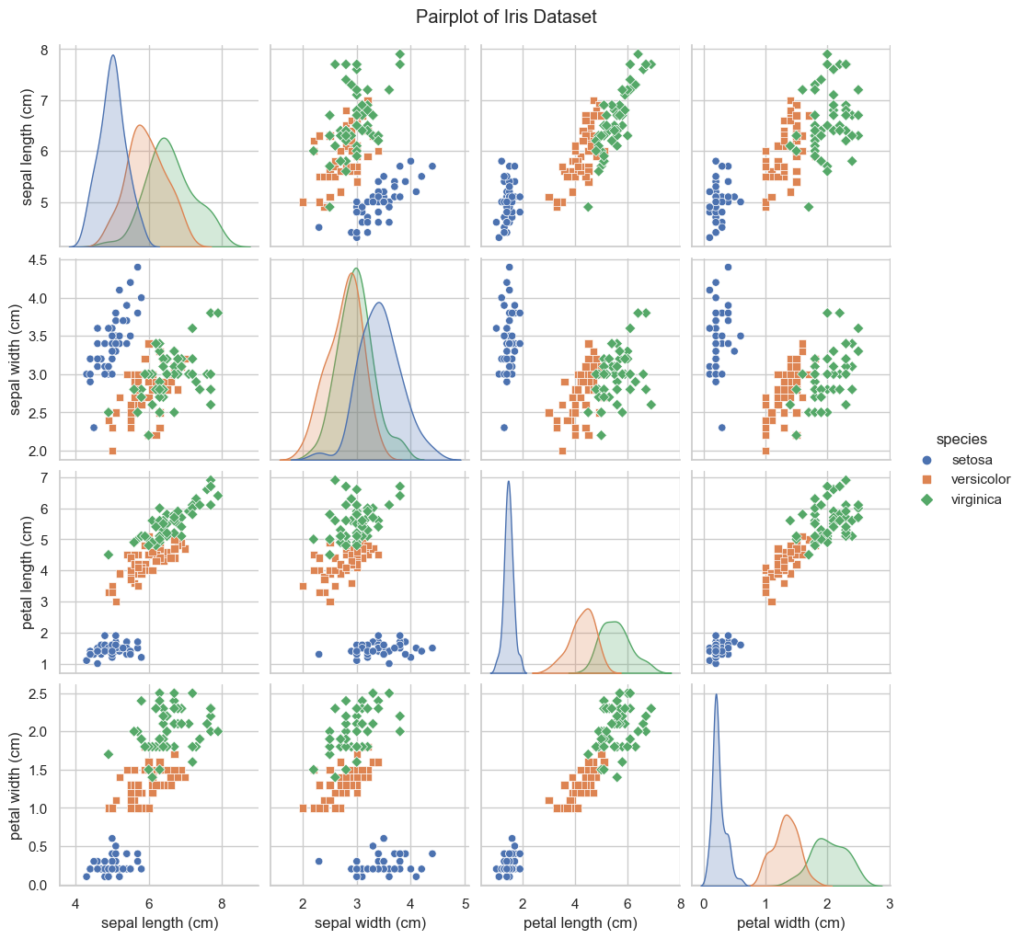
The pairplot above provides a pairwise relationship between all numerical variables. Different colors represent different species of the Iris flower.
- Diagonal: The diagonal shows the distribution of a single variable for each species. We can see that the Setosa species is easily distinguishable from the others based on petal length and petal width.
- Off-diagonal: The off-diagonal plots show scatter plots between two variables. These can help us understand the correlation between two variables for each species.
Step 4: Statistical Summary
Let’s take a closer look at the statistical distribution of the features across the different species.
# Group the data by species and calculate the mean and standard deviation for each group
grouped_mean = iris_df.groupby('species').mean()
grouped_std = iris_df.groupby('species').std()

grouped_mean, grouped_std
Output:
(            sepal length (cm)  sepal width (cm)  petal length (cm)  \
 species
 setosa                  5.006             3.428              1.462
 versicolor              5.936             2.770              4.260
 virginica               6.588             2.974              5.552

             petal width (cm)
 species
 setosa                 0.246
 versicolor             1.326
 virginica              2.026  ,
             sepal length (cm)  sepal width (cm)  petal length (cm)  \
 species
 setosa               0.352490          0.379064           0.173664
 versicolor           0.516171          0.313798           0.469911
 virginica            0.635880          0.322497           0.551895

             petal width (cm)
 species
 setosa              0.105386
 versicolor          0.197753
 virginica           0.274650  )
The table below summarizes the mean and standard deviation of each feature for the different species:
| Feature | Setosa (Mean) | Versicolor (Mean) | Virginica (Mean) | Setosa (Std) | Versicolor (Std) | Virginica (Std) |
|---|---|---|---|---|---|---|
| Sepal length (cm) | 5.006 | 5.936 | 6.588 | 0.352 | 0.516 | 0.636 |
| Sepal width (cm) | 3.428 | 2.770 | 2.974 | 0.379 | 0.314 | 0.322 |
| Petal length (cm) | 1.462 | 4.260 | 5.552 | 0.174 | 0.470 | 0.552 |
| Petal width (cm) | 0.246 | 1.326 | 2.026 | 0.105 | 0.198 | 0.275 |
- Setosa: Generally has smaller dimensions.
- Versicolor: Has dimensions that are intermediate between Setosa and Virginica.
- Virginica: Generally has larger dimensions.
Step 5: Correlation Analysis of Iris Dataset
Finally, let’s check how the features correlate with each other.
# Calculate the correlation matrix
correlation_matrix = iris_df.corr()

# Generate a heatmap to visualize the correlation matrix
plt.figure(figsize=(10, 8))
sns.heatmap(correlation_matrix, annot=True, cmap='coolwarm', fmt=".2f")
plt.title('Correlation Heatmap of Iris Dataset')
plt.show()
Output:

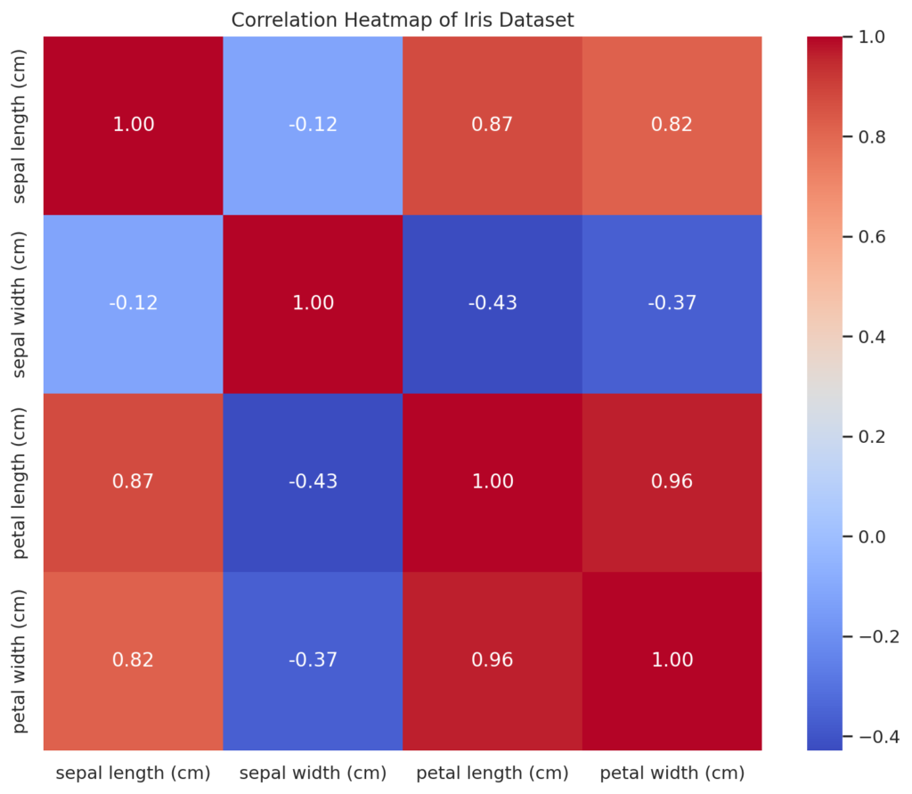
The heatmap above shows the correlation matrix for the feature variables in the Iris dataset. The values range from -1 to 1, with -1 indicating a strong negative correlation, 1 indicating a strong positive correlation, and 0 indicating no correlation.
Here are some observations:
- Sepal Length is positively correlated with Petal Length and Petal Width, suggesting that longer sepals are associated with longer and wider petals.
- Sepal Width shows relatively low correlation with other features.
- Petal Length and Petal Width are strongly positively correlated, indicating that longer petals are generally also wider.
That wraps up our complete data analysis and visualization of the Iris dataset.


