Data Analysis for Titanic Dataset

The Titanic dataset is a popular dataset used for data analysis and machine learning. It contains information about the passengers onboard the RMS Titanic, which tragically sank on April 15, 1912. The dataset is often used for predictive modeling, to predict who survived or died in the disaster. In this article we shall provide a complete data analysis for Titanic dataset.

Table of Contents

• Data Exploration
• Data Cleaning
• Data Analysis
• Data Visualization
• Summary of Findings

To conduct a complete data analysis for Titanic dataset, we’ll proceed with the following steps:

1. Data Exploration: Understand the structure of the data.
2. Data Cleaning: Clean the data for missing or irrelevant values.
3. Data Analysis: Conduct descriptive statistics to summarize the data.
4. Data Visualization: Create visualizations to better understand the data.
5. Summary: Sum up the findings.

Let’s start by exploring the data.

Packages required: pandas, matplotlib, seaborn

Dataset: download titanic.csv

# Importing necessary libraries
import pandas as pd

# Load the downloaded Titanic dataset
file_path = 'Titanic.csv'
titanic_data = pd.read_csv(file_path)

# Show the first few rows of the dataset to get an overview
titanic_data.head()

Output:

PassengerId	Survived	Pclass	Name	                       Sex	   Age	SibSp	Parch	 Ticket	         Fare	   Cabin	  Embarked
	1	           0	      3	   Braund, Mr. Owen Harris	     male	   22.0	  1	   0	    A/5 21171	     7.2500	  NaN	      S
	2	           1	      1	   Cumings, Mrs. John Bradley    female	 38.0	  1	   0	    PC 17599	     71.2833	C85	      C
	3	           1	      3	   Heikkinen, Miss. Laina	       female	 26.0	  0	   0	   STON/O2.3101282 7.9250	  NaN	      S
	4	           1	      1	   Futrelle, Mrs. Jacques Heath  female	 35.0	  1	   0	   113803	         53.1000	C123	    S
	5	           0	      3	   Allen, Mr. William Henry	     male	   35.0	  0	   0	   373450	         8.0500	  NaN	      S

Data Exploration

The dataset contains the following columns:

1. Sex: Gender of the passenger (male/female)
2. Age: Age of the passenger
3. SibSp: Number of siblings/spouses aboard
4. Parch: Number of parents/children aboard
5. Fare: Ticket fare
6. Embarked: Port of embarkation (C = Cherbourg; Q = Queenstown; S = Southampton)
7. Pclass: Ticket class (First, Second, Third)
8. Cabin: cabin number
9. Survived: Whether the passenger survived (1) or not (0)

Let’s check for missing values and data types before proceeding further.

# Check for missing values and data types of each column
import pandas as pd
missing_values = titanic_data.isnull().sum()
data_types = titanic_data.dtypes

missing_values_df = pd.DataFrame({'Missing Values': missing_values, 'Data Type': data_types})
missing_values_df

Missing     Values	Data Type
PassengerId	  0	    int64
Survived	    0	    int64
Pclass	      0	    int64
Name	        0	    object
Sex	          0	    object
Age	          177	  float64
SibSp	        0  	  int64
Parch	        0	    int64
Ticket	      0	    object
Fare	        0	    float64
Cabin	      687	    object
Embarked	    2	    object

Data Cleaning

We have the following issues in the dataset:

1. age: 177 missing values
2. embarked: 2 missing values

To handle these:

• For the age column, we can fill the missing values with the median age.
• For the embarked column, we can fill the missing values with the most frequent port of embarkation.

Let’s proceed with the data cleaning.

# Fill missing values in the 'age' column with the median age
median_age = titanic_data['Age'].median()
titanic_data['Age'].fillna(median_age, inplace=True)

# Fill missing values in the 'embarked' column with the most frequent value
most_frequent_embarked = titanic_data['Embarked'].mode()[0]
titanic_data['Embarked'].fillna(most_frequent_embarked, inplace=True)

# Verify that there are no more missing values
titanic_data.isnull().sum()

PassengerId      0
Survived         0
Pclass           0
Name             0
Sex              0
Age              0
SibSp            0
Parch            0
Ticket           0
Fare             0
Cabin          687
Embarked         0

Data Cleaning Summary

All missing values have been successfully addressed:

• The age column’s missing values have been filled with the median age.
• The embarked column’s missing values have been filled with the most frequent port of embarkation.

# Calculate basic statistical measures for the numerical columns
statistical_summary = titanic_data.describe()

statistical_summary

            Age       SibSp       Parch        Fare    Survived
count  891.000000  891.000000  891.000000  891.000000  891.000000
mean    29.361582    0.523008    0.381594   32.204208    0.383838
std     13.019697    1.102743    0.806057   49.693429    0.486592
min      0.420000    0.000000    0.000000    0.000000    0.000000
25%     22.000000    0.000000    0.000000    7.910400    0.000000
50%     28.000000    0.000000    0.000000   14.454200    0.000000
75%     35.000000    1.000000    0.000000   31.000000    1.000000
max     80.000000    8.000000    6.000000  512.329200    1.000000

Data Analysis

Let’s now proceed with some basic statistical analysis to summarize the dataset.

Data Analysis Summary

Here are some key statistical insights about the numerical columns:

1. Age: The average age of passengers is approximately 29.36 years, with a standard deviation of 13.02. The youngest passenger was 0.42 years old, and the oldest was 80.
2. SibSp (Siblings/Spouses): On average, passengers had about 0.52 siblings or spouses aboard. The maximum number in this category is 8.
3. Parch (Parents/Children): On average, passengers had about 0.38 parents or children aboard. The maximum number in this category is 6.
4. Fare: The average ticket fare was approximately 32.20 units, with a wide standard deviation of 49.69. The fare ranged from 0 to 512.33 units.
5. Survived: About 38.4% of the passengers in this dataset survived.

Data Visualization

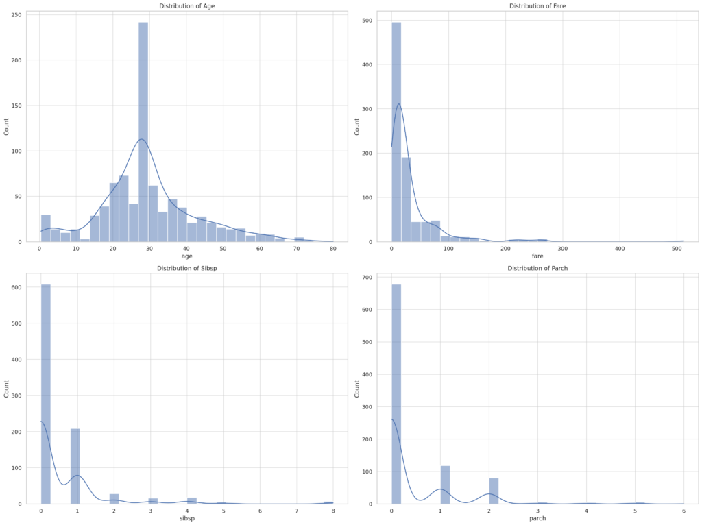
Let’s now visualize the data to uncover more insights. We’ll look at:

• Distribution of numerical features
• Categorical features vs Survival rate
• Correlations between features

Let’s start by visualizing the distribution of numerical features like age, fare, siblings/spouses, and parents/children.

# Importing necessary libraries for data visualization
import matplotlib.pyplot as plt
import seaborn as sns

# Set the style for the visualizations
sns.set(style="whitegrid")

# Initialize the figure
plt.figure(figsize=(20, 15))

# Create a list of numerical features
numerical_features = ['Age', 'Fare', 'SibSp', 'Parch']

# Create subplots for each numerical feature
for i, feature in enumerate(numerical_features, 1):
    plt.subplot(2, 2, i)
    sns.histplot(titanic_data[feature], bins=30, kde=True)
    plt.title(f'Distribution of {feature.capitalize()}')

plt.tight_layout()
plt.show()

Data Visualization Summary: Numerical Features

1. Age: The age distribution is somewhat skewed to the right, with a higher concentration of passengers between 20 and 30 years old.
2. Fare: The fare distribution is highly skewed to the right, indicating that most passengers paid a lower fare, while a few paid extremely high fares.
3. SibSp (Siblings/Spouses): Most passengers did not have siblings or spouses aboard, as indicated by the peak at 0.
4. Parch (Parents/Children): Similar to SibSp, most passengers did not have parents or children aboard.

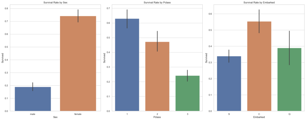
Next, let’s examine how categorical features like sex, class, and port of embarkation relate to the survival rate.

# Initialize the figure
plt.figure(figsize=(20, 15))

# Create a list of categorical features related to survival
categorical_features = ['Sex', 'Class', 'Embarked']

# Create subplots for each categorical feature vs survival
for i, feature in enumerate(categorical_features, 1):
    plt.subplot(2, 3, i)
    sns.barplot(x=feature, y='survived', data=titanic_data)
    plt.title(f'Survival Rate by {feature.capitalize()}')

plt.tight_layout()
plt.show()

Data Visualization Summary: Categorical Features vs Survival

1. Sex: Females had a significantly higher survival rate compared to males.
2. Class: Passengers in the First Class had the highest survival rate, followed by those in the Second Class and Third Class.
3. Embarked: Passengers who embarked at Cherbourg (C) had the highest survival rate, followed by those from Queenstown (Q) and Southampton (S).

Summary of Findings

1. The dataset had some missing values in the ‘age’ and ’embarked’ columns, which were successfully handled.
2. Age, Fare, and family size (SibSp, Parch) were distributed unevenly, with most passengers being young adults, paying low fares, and traveling without family.
3. Survival rates varied significantly based on sex, class, point of embarkation, and whether the passenger was alone.